Differential Geometry Part VI: Geometry of Surfaces in Euclidean Space
July 18th, 2017
We continue by analogy. First, we set up the essential machinery for discussing curves in $\mathbb{R}^3$, such as frame fields, connection forms, and the structural equations in Part II. Then in Part III, we discussed the geometry of $\mathbb{R}^3$, or more specifically, the unique properties which are preserved by Euclidean isometries. Similarly, in Part V we discussed the machinery for discussing surfaces in $\mathbb{R}^3$, namely the shape operator. And in Part VI we will discuss the intrinsic geometry of a surface in $\mathbb{R}^3$, concluding as we did Part III with a congruence theorem for surfaces. Man, it’s like poetry. Makes me tear up.
The Fundamental Equations
Once more, the Cartan equations from Part II find their use. As with the Frenet frame approach, we first need to set up a system of frames on $M$.
Definition: An adapted frame field $E_i$ on a region $\mathcal{O}$ in $M \subset \mathbb{R}^3$ is a Euclidean frame field (three orthonormal vector fields) such that $E_3$ is always normal to $M$.
Lemma
On a region $\mathcal{O}$ in $M \subset \mathbb{R}^3$, there exists an adapted frame field if and only if $\mathcal{O}$ is orientable and there exists a non-vanishing tangent vector field on $\mathcal{O}$.
This condition is clearly necessary, since the orientable condition guarantees the existence of a unit normal vector field (see: Part IV), and the tangent space condition guarantees us the remaining two vector fields. From a unit vector field $U$ and a tangent vector $V$, we can define a frame:
$$\begin{aligned} E_1 &= \frac{V}{\vert V \vert} \\ E_2 &= U \times E_1 \\ E_3 &= U \end{aligned}$$
This lemma immediately implies that on the image of any patch in $M$, there is an adapted frame field on $M$ in an open region. Thus adaptable frame fields exist on surfaces, at least locally.
Suppose $E_i$ are an adapted frame field on $M$. We can extend the frame field so that it is defined on an open set in $\mathbb{R}^3$. Now, we look at the connection equations:
$$\begin{aligned} \nabla_v E_i = \sum \omega_{ij}(v) E_j \end{aligned}$$
This definition really only makes sense if we apply them to tangent vectors $v$ to $M$. Now, we have a set of $1$-forms defined on $M$.
Again, $\omega_{ij}(v)$ defines the initial rate at which $E_i$ rotates towards $E_j$ as $p$ moves in the direction $v$.
Corollary
As a corollary, we can define the shape operator in terms of the connection forms, since $E_3 = U$ is a unit normal vector field. Then:
$$\begin{aligned} S_p(v) = \omega_{13}(v)E_1(p) + \omega_{23}E_2(p) \end{aligned}$$
This follows directly from the connection equations.
We also can carry over directly the dual $1$ -forms, $\theta_i(v) = v\cdot E_i$, as long as we restrict $v$ to tangent vectors to $M$. This means that in particular, $\theta_3(v) = 0$, since $E_3$ does not lie in the tangent plane. Thus, due to skew-symmetry, we essentially only have five $1$-forms:
- $\theta_1, \theta_2$ are dual to the tangent vector fields $E_1, E_2$.
- $\omega_{12}$ gives the rate of rotation of $E_1$ towards $E_2$.
- $\omega_{13}, \omega_{23}$ completely describe the shape operator.
Theorem
The big one! If $E_i$ is an adapted frame field on $M \subset \mathbb{R}^3$, then its dual forms and connection forms satisfy:
First Structural Equations
$$\begin{aligned} d \theta_1 &= \omega_{12} \wedge \theta_2 \\ d \theta_2 &= \omega_{21} \wedge \theta_1 \end{aligned}$$
Gauss Equation
$$\begin{aligned} d \omega_{12} = \omega_{13} \wedge \omega_{32} \end{aligned}$$
Codazzi Equations
$$\begin{aligned} d \omega_{13} = \omega_{13} \wedge \omega_{23} \\ d \omega_{23} = \omega_{21} \wedge \omega_{13} \end{aligned}$$
The first structural equations are the same as in Part II. The second structural equations imply the Gauss equations and the Codazzi equations, the former of which describes the rotation between $E_1, E_2$ and the latter of which describes the shape operator. It is important to note that these equations depend on the choice of frame field.
Since the corresponding connection forms describe the shape operator, the Codazzi equations describe the rate at which the shape of $M$ is changing.
Lemma
We can describe geodesics using connection forms. Let $\alpha$ be a unit speed curve in $M$. If $E_1, E_2, E_3$ is an adapted frame field where $E_1 = T$ along $\alpha$ ($T$ being the unit tangent vector from the Frenet frame), we claim that $\alpha$ is a geodesic if and only if $\omega_{12}(T) = 0$.
First, denote $E_i’ = E_i(\alpha(t))$ at $t=0$. But this is the same as the covariant derivative: $E_i’ = \nabla_{\alpha’} E_i$. In particular for this curve, $\alpha’ = T$.
Since $E_i$ is an adapted frame field and $T$ is a unit vector, $E_i’$ must be entirely in the diretction of $E_2$. This means that: $\omega_{12}(T) = (\nabla_T E_1) \cdot E_2$. But since $\alpha$ is a geodesic, $\alpha’’$ is normal to $M$; so there is no such component in the $E_2$ direction, so indeed $\omega_{12}(T) = 0$.
So, the connection forms already find some use in making sense of curves on surfaces.
Form Computations
If $E_1, E_2, E_3$ is an adapted frame field on $M \subset \mathbb{R}^3$, we say that $E_1, E_2$ constitute a tangent frame field on $M$. So any tangent vector field $V$ on $M$ can be decomposed into its components $V \cdot E_1, V\cdot E_2$ along each of the tangent frames.
Thus, to show that two forms are equal, we just have to compare them on basis vector fields $E_1, E_2$. So now we can equivalently form a “basis” of forms on $M$.
Lemma
Let $\theta_1, \theta_2$ be the dual $1$-forms of $E_1, E_2$ on $M$. If $\phi$ is a $1$-form and $\psi$ a $2$-form, then:
$$ \phi = \phi(E_1) \theta_1 + \phi(E_2) \theta_2 $$
$$ \mu = \mu(E_1, E_2) \theta_1 \wedge \theta_2 $$
The first statement comes easily from the criteria for equality of frame fields; the second comes from our definition of the wedge product:
$$\begin{aligned} \theta_1 \wedge \theta_2(E_1, E_2) &= \theta_1(E_1) \theta_2(E_2) - \theta_1 (E_2) \theta_2 (E_1) \\ &= 1 \end{aligned}$$
Lemma
$$ \omega_{13} \wedge \omega_{23} = K \theta_1 \wedge \theta_2 $$
$$ \omega_{13} \wedge \theta_2 + \theta_1 \wedge \omega_{23} = 2H \theta_1 \wedge \theta_2 $$
To prove these equations, first we need to write a matrix representation of the shape operator $S$. From the connection equations:
$$\begin{aligned} S(E_1) &= -\nabla_{E_1} E_3 = \omega_{13}(E_1) E_1 + \omega_{23}(E_1) E_2 \\ S(E_2) &= -\nabla_{E_2} E_3 = \omega_{13}(E_1) E_1 + \omega_{23}(E_1) E_2 \end{aligned}$$
So the matrix of $S$ is then:
$$ \begin{bmatrix} \omega_{13} (E_1) & \omega_{13} (E_2)\\ \omega_{23} (E_1) & \omega_{23} (E_2) \end{bmatrix}$$
Now, we test equality of forms in the usual way. For the first form:
$$\begin{aligned} (\omega_{13} \wedge \omega_{23})(E_1, E_2) &= \omega_{13}(E_1)\omega_{23}(E_2) - \omega_{13}(E_2) \omega_{23}(E_1) \\ &= \det S \\ &= K \end{aligned}$$
And similarly for the second form:
$$\begin{aligned} (\omega_{13}\wedge \theta_2 + \theta_1\wedge \omega_{23})(E_1, E_2) &= \omega_{13}(E_1) + \omega_{23}(E_2) \\ &= \text{tr} S \\ &= 2H \end{aligned}$$
And from the first half of this lemma and the Gauss equation, we get:
$$\begin{aligned} d \omega_{12} = -K \theta_1 \wedge \theta_2 \end{aligned}$$
Which we will call the second structural equation. Since $\omega_{12}$ is something like the rate of rotation of the tangent frame field $E_1, E_2$, its derivative $K$ measures something like a second derivative of $E_1, E_2$.
Definition: A principal frame field on $M$ is an adapted frame field so that $E_1, E_2$ are principal vectors of $M$.
Where there are no umbilic points, there is a unique principal frame on $M$ up to changes in sign. We leave this proof out, but it’s not hard to prove using linear algebra and some analysis.
Suppose we have a principal frame field on $M$, then we can rename the principal directions so that $S(E_1) = k_1 E_1$ and $S(E_2) = k_2 E_2$. Thus by the basis formula from earlier, we have:
$$\begin{aligned} \omega_{13} &= k_1 \theta_1 \\ \omega_{23} &= k_2 \theta_2 \end{aligned}$$
This leads us to an interesting corollary of the Codazzi equations.
Theorem
If $E_1, E_2, E_3$ is a principal frame field on $M$, then:
$$\begin{aligned} E_1[k_2] = (k_1 - k_2) \omega_{12}(E_2) \\ E_2[k_1] = (k_1 - k_2) \omega_{12}(E_1) \end{aligned}$$
We can prove this just with differential forms algebra. First, we apply the Codazzi equations:
$$\begin{aligned} d(\omega_{13}) = d(k_1 \theta_1) & =\omega_{12} \wedge \omega_{23} \\ dk_1 \wedge \theta_1 + k_1 d\theta_1 &= k_2 \omega_{12} \wedge \theta_2 \\ \end{aligned}$$
But we also know from the First Structural Equations that $d \theta_1 = \omega_{12} \wedge \theta_2$. So finally we have:
$$\begin{aligned} dk_1 \wedge \theta_2 = (k_2 - k_1) \omega_{12} \wedge \theta_2 \end{aligned}$$
To prove this statement, we simply apply each of the $2$-forms to $(E_1, E_2)$:
$$\begin{aligned} (dk_1 \wedge \theta_2)(E_1, E_2) &= (k_2 - k_1) \omega_{12} \wedge \theta_2 (E_1, E_2) \\ -dk_1(E_2) &= (k_2 - k_1) \omega_{12} (E_1) \end{aligned}$$
Therefore:
$$\begin{aligned} E_2[k_1] = dk_1(E_2) = (k_1 - k_2) \omega_{12} (E_1) \end{aligned}$$
And similarly for the second statement.
Some Global Theorems
We know apply our knowledge of the shape operator to draw some conclusions of (connected) surfaces.
Theorem
If $S$ is identically zero, then $M$ is part of the plane in $\mathbb{R}^3$.
This means that the unit vector field $E_3$ is the same vector everywhere. So, we pick a fixed point $p$ in $M$ and consider any other point $q$ in $M$, and draw a curve $\alpha$ in $M$ so that $\alpha(0) = p, \alpha(1) = q$. So we consider the function:
$$\begin{aligned} f(t) &= (\alpha(t) - p)\cdot E_3 \\ \frac{df}{dt} &= \alpha' \cdot E_3 = 0 \end{aligned}$$
So indeed, since $f(0) = 0$, $f$ is identically zero. By checking $f(1)$, we see that indeed $(q-p)\cdot E_3 = 0$, so that indeed, $q$ lies in the plane normal to $E_3$.
Theorem
If $M$ is umbilic everywhere, then $M$ has constant Gaussian curvature.
To prove this, for each region in $M$ we pick an adapted frame field $E_1, E_2, E_3$. Since every direction is a principal direction, indeed this is a principal frame field. So our earlier lemma from the Codazzi equations in the previous section, we have:
$$\begin{aligned} dk(E_1) = dk(E_2) = 0 \end{aligned}$$
By the basis formulas, $dk = 0$ in the region. But then we know that $dK = d(k_1^2) = 2k_1 dk$ = 0. So indeed, we have shown that $K$ is constant everywhere since $dK=0$ in every region of $M$.
Theorem
If $M$ is umbilic everywhere, and $K > 0$, then $M$ is part of a sphere in $\mathbb{R}^3$ of radius $\frac{1}{\sqrt{K}}$.
To prove this theorem, We will construct a point which is equidistant from every point in $M$. Pick any point $p$ of $M$ and denote the unit normal $E_3$. Then we claim that the center is:
$$\begin{aligned} c = p + \frac{1}{k(p)} E_3(p) \end{aligned}$$
Now, we pick any point $q$ of $M$, and draw a curve $\alpha$ in $M$ as in the preceding proof with $\alpha(0) = p, \alpha(1) =q$. We extend $E_3$ to a unit normal vector field all along $\alpha$. Now all we have to do is consider the curve:
$$\begin{aligned} \gamma = \alpha + \frac{1}{k} E_3 \end{aligned}$$
How do we know $k$ is a constant? Well, since $E_3$ was extended continuously, $k(p)$ is also continuous; but our previous theorem tells us that the Gaussian curvature $K=k^2$ is constant. Taking the derivative of $\gamma$, we get:
$$\begin{aligned} \gamma' = \alpha' + \frac{1}{k} E_3' \end{aligned}$$
But by the definition of the shape operator (which we recall is just scalar multiplication at umbilic points):
$$\begin{aligned} E_3' = -S(\alpha') = -k\alpha' \end{aligned}$$
So indeed $\gamma’ = 0$, and $\gamma$ is constant. So in particular:
$$\begin{aligned} \gamma(0) = p +\frac{1}{k}E_3 = \gamma(1) = q+\frac{1}{k}E_3 \end{aligned}$$
And in particular, $\vert c-p \vert = \vert c - q \vert$. Furthermore, since $K = k^2$, the distance is indeed $\frac{1}{\sqrt{K}}$.
Combining the three previous theorems: A surface is all-umbilic if and only if $M$ is a part of a plane or sphere.
Corollary
A compact all-umbilic surface is a sphere.
First, we note from topology that a connected space has only two clopen sets: the empty set, and the whole space. In particular, both planes and spheres are connected.
Now, if $M$ is compact, then it is automatically closed and bounded. Furthermore, for each patch in $M$, since $x$ is continuous with continuous inverse, open sets map to open sets. Suppose that $M \subset N$ for some other surface $N$; then this means $M$, being the union of a collection of patches, is indeed a collection of open sets and thus open. Since $M$ is open and closed in a connected surface $N$, it is either empty, or all of $N$ itself.
If $M$ is compact, it can’t be a plane; therefore it must be a sphere.
Before proceeding into the next theorem, we first prove a useful lemma which relates the Gaussian curvature to the connection forms. First, by the basis theorem, we can write:
$$\begin{aligned} \omega_{12} = \omega_{12}(E_1) \theta_1 + \omega_{12}(E_2) \theta_2 \end{aligned}$$
And we also have from an earlier lemma:
$$\begin{aligned} d \omega_{12} = -K \theta_1 \wedge \theta_2 \end{aligned}$$
So, we differentiate each term in the earlier expansion of $\omega_{12}$:
$$\begin{aligned} d \omega_{12} = d \omega_{12}(E_1) \wedge \theta_1 &+ \omega_{12}(E_1) d\theta_1 \\ +d \omega_{12}(E_2) \wedge \theta_2 &+ \omega_{12}(E_2) d\theta_2 \end{aligned}$$
But the first structural equations allow us to write $d\theta_i$. And indeed if we apply the $2$-form above to the pair $(E_1, E_2)$, we arrive at:
$$\begin{aligned} K = -d\omega_{12} (E_1, E_2) = E_2[\omega_{12}(E_1)] - E_1[\omega_{12}(E_2)] - \omega_{12}(E_1)^2 - \omega_{12}(E_2)^2 \end{aligned}$$
This puts Gaussian curvature entirely in terms of covariant derivatives and connection forms.
Theorem
On every compact surface $M$ in $\mathbb{R}^3$, there is a point at which the Gaussian curvature $K$ is strictly positive.
We consider the real-valued (differentiable) function $f(p) = p\cdot p$ on a compact surface. Since $M$ is compact, $f$ attains a maximum at some point $m$ on $M$$
Take any unit tangent vector $u$ to $M$ at $m$, and pick a unit curve $\alpha$ on $M$ so that $\alpha(0)=m, \alpha’(0)=u$. Then indeed, $f(\alpha(t))$ also has a maximum there, i.e.:
$$\begin{aligned} \frac{d}{dt}(f\circ \alpha) (0) &= 0 \\ \frac{d^2}{dt^2}(f\circ \alpha) (0) \le 0 \end{aligned}$$
But we note that by our definition, $\frac{d}{dt}(f\circ \alpha) = 2\alpha \cdot \alpha$. So indeed:
$$\begin{aligned} \frac{d}{dt}(f\circ \alpha) (0) &= 0 = 2(m\cdot u) \end{aligned}$$
So this means that $m$ is normal to $M$, since it is perpendicular to any tangent vector, and this means that locally, $M$ looks like a sphere. Differentiating again:
$$\begin{aligned} \frac{d^2}{dt^2}(f\circ \alpha) (0) &= 2\alpha' \cdot \alpha' + 2\alpha \cdot \alpha'' \\ &= 2(1 + m\cdot \alpha''(0)) \le 0 \end{aligned}$$
Where the second equality comes from evaluating at $t=0$.
Now, earlier we proved that $m$ is a normal to $M$, so all we have to do is divide by its length $r$ to get a unit normal vector. Thus, $m/r \cdot \alpha’’$ is exactly the normal curvature $k(u)$ (See: Part V, Normal Curvature). So our inequality then becomes:
$$\begin{aligned} k(u) \le \frac{1}{r} \end{aligned}$$
Since both principal curvatures satisfy this inequality, we have:
$$\begin{aligned} K(m) \ge \frac{1}{r^2} > 0 \end{aligned}$$
So we have shown there is a point where the Gaussian curvature is positive.
Corollary
As an immediate corollary, there is no compact surface in $\mathbb{R}^3$ with $K \le 0$. So if we have a compact surface with constant Gaussian curvature, it must be positive. A sphere is an example of such a surface – and, as it turns out, it is the only example. To prove this, we begin wth a lemma.
Lemma
Let $m$ be a point in $M$ so that:
- $k_1$ achieves its local maximum at $m$.
- $k_2$ achieves its local minimum at $m$.
- $k_1(m) > k_2(m)$
Then, $K(m) \le 0$.
Proof
First, if $f$ is a differentiable function on $M$ and $V$ a vector field, then we have also a first derivative $V[f]$ which yields a second derivative $VV[f] = V[V[f]]$. At a local maximum, it is not hard to prove that $V[f] = 0$ and $VV[f] \le 0$, just as in calculus.
Now since $k_1 > k_2$ at $m$, and this is a strict inequality, then $m$ is not umbilic; so there exists a principal frame field $E_1, E_2, E_3$ on a neighborhood of $m$, and indeed by calculus:
$$\begin{aligned} E_1[m] = E_2[m] &= 0 \\ E_1E_1[k_2] \ge 0 \\ E_2E_2[k_1] \le 0 \\ \end{aligned}$$
Where the inequality follows from the fact that $k_2$ achieves a minimum, and $k_2$ a maximum. Now we apply the Codazzi equations in the way they appear on a principal frame field, and discover that at $m$:
$$\begin{aligned} \omega_{12}(E_1) = \omega_{12}(E_2) = 0 \end{aligned}$$
Now, by an earlier lemma:
$$\begin{aligned} K &= E_2[\omega_{12}(E_1)] - E_1[\omega_{12}(E_2)] - \omega_{12}(E_1)^2 - \omega_{12}(E_2)^2 \\ &= E_2[\omega_{12}(E_1)] - E_1[\omega_{12}(E_2)] \end{aligned}$$
To understand these terms, we apply $E_i$ to the Codazzi equations to derive the inequalities:
$$\begin{aligned} E_1[\omega_{12}(E_2)] \ge 0 \\ E_2[\omega_{12}(E_1)] \le 0 \end{aligned}$$
And thus our earlier expression for $K$ reveals that indeed, $K \le 0$.
Theorem
Now we’re finally ready to prove the theorem that a compact surface in $\mathbb{R}^3$ with constant Gaussian curvature is indeed a sphere of radius $\frac{1}{\sqrt{K}}$
Since the surface is compact, it is orientable, giving us a continuous shape operator and continuous principal curvatures $k_1, k_2$. Since $M$ has constant Guassian curvature, we earlier proved that $K > 0$. Since we’re working on a compact surface, $k_1$ has a maximum at some point $p$. Since $K$ is constant, that also means $k_2$ is at a maximum.
From the immediately preceding lemma, the only missing condition is that $k_1 > k_2$ at $p$; if that were true, then $K \le 0$, which is a contradiction. So we know that $k_1 = k_2$, not just at this point, but everywhere. So $M$ is all-umbilic and it is therefore a sphere.
Note that compactness is essential for this proof.
Isometries and Local Isometries
Definition: If $p,q$ are points in $M$, we consider all the curves $\alpha$ from $p$ to $q$. The intrinsic distance $\rho(p,q)$ is the greatest lower bound on the lengths $L(\alpha)$ of the curves.
Note that this is just a greatest lower bound; there is not necessarily an actual curve with that length (due to limits). Now that we have a “metric”, we can define an isometry.
Definition: An isometry $F:M\rightarrow \bar{M}$ of surfaces in $\mathbb{R}^3$ is a one-to-one mapping from $M$ onto $\bar{M}$ that preserves dot products of tangent vectors. Explicitly:
$$\begin{aligned} F_\star(v) \cdot F_\star(w) = v \cdot w \end{aligned}$$
Note that this was a theorem in Part III; the tangent map of an isometry in Euclidean space is simply its orthogonal component, evaluated at $F(p)$, and therefore dot products are preserved. Along with dot products, of course, we get lengths and orthogonality. It follows that isometries are regular mappings (its tangent map is one-to-one), because the tangent map sends zero vectors to zero vectors; and indeed this means that by the inverse function theorem, $F$ is a diffeomorphism, i.e. has an inverse mapping (which is also an isometry).
Theorem
Isometries preserve intrinsic distance.
We would hope that this holds. To prove this, consider any curve and recall how we defined its arclength by integrating its speed. Well, for any curve $\alpha$, $\alpha’$ is a tangent vector; thus isometries preserve the norm of $\alpha’$ (speed), and therefore preserve arclength.
If there is an isometry between two surfaces, we call them isometric; for example, bending a piece of paper without stretching, folding, or tearing is an isometry.
Definition: A local isometry $F:M\rightarrow N$ of surfaces is a mapping that preserves dot products of tangent vectors.
Thus a local isometry need not be one-to-one and onto, and thus $F$ is not necessarily a diffeomorphism. However, since $F$ is regular on some neigborhood of any point, $F$ carries that neigborhood diffeomorphically to a neighborhood of $F(p)$. Indeed, a local isometry works like an isometry, but only locally.
Lemma
Let $F:M\rightarrow N$ be a mapping. For each patch $x: D\rightarrow M$, we consider the composite mapping:
$$\begin{aligned} \bar{x} = F(x): D \rightarrow N \end{aligned}$$
Then, $F$ is a local isometry if and only if for each patch $x$ we have:
$$\begin{aligned} E &= \bar{E} \\ F &= \bar{F} \\ G &= \bar{G} \end{aligned}$$
We prove both directions simultaneously.
First, recognize that we only need to show that $F_\star$ preserves dot products between $x_u, x_v$. The curve $\alpha = x(u,v_0)$ for which $\alpha’=x_u$ gets sent by $F$ to $F\circ \alpha$, a curve in $N$ for which $(F\circ \alpha)’ = \bar{x_u}$, So indeed:
$$\begin{aligned} F_\star(x_u) = \bar{x_u} \\ F_\star(x_v) = \bar{x_v} \end{aligned}$$
And since $F$ is a local isometry, it therefore preserves dot products and therefore $E,F,G$. Reversing this argument, we deduce the converse statement; the tangent map preserves dot products, therefore it is a local isometry.
We can use this theorem to construct local isometries. Suppose we have $x:D\rightarrow M$ and $y:D\rightarrow N$. Then we can construct a mapping:
$$\begin{aligned} F(x(u,v)) = y(u,v) \end{aligned}$$
And if $E = \bar{E}, F=\bar{F}, G=\bar{G}$, then $F$ is a local isometry.
Definition: A mapping of surfaces $F:M\rightarrow N$ is conformal provided there exists a real-valued function $\lambda > 0$ on $M$ such that:
$$\begin{aligned} \vert F_\star(v_p) \vert = \lambda(p) \vert v(p) \vert \end{aligned}$$
The function $\lambda$ is called a scale factor for $F$. This is a generalization of a local isometry where dot products are not preserved, but at a certain point the tangent vectors are all stretched by the same factor.
Intrinsic Geometry of Surfaces in $\mathbb{R}^3$
As before, we wish to study the properties of surfaces preserved by isometries, but not by arbitrary mappings. First note that since dot products are preserved, we still have tangent frames. From an adapted frame field we still have $E_1, E_2$ and their dual forms. What else can we say?
Lemma
The connection form $\omega_{12}$ is the only $1$-form that satisfies the first structural equations:
$$\begin{aligned} d\theta_1 &= \omega_{12} \wedge \theta_2 \\ d\theta_2 &= \omega_{21} \wedge \theta_1 \end{aligned}$$
To prove this, we apply the wedge products on the RHS to the pair of tangent vector fields $E_1, E_2$:
$$\begin{aligned} d\theta_1(E_1, E_2) &= \omega_{12}(E_1) \\ d\theta_2(E_1, E_2) &= \omega_{21}(E_2) = -\omega_{12}(E_2) \end{aligned}$$
Thus, by the basis lemma, the connection form $\omega_{12}$ is completely determined by $\theta_1, \theta_2$, which as we said before, is preserved by isometries. In fact, we can regard the above lemma as the definition of the connection forms, and it has nothing to do with the shape operator or covariant derivatives, just differential forms.
If $F:M\rightarrow \bar{M}$ is an isometry, we transfer the tangent frame $E_1, E_2$ at $p$ to the pair $\bar{E_1}, \bar{E_2} = F_\star(E_1), F_\star(E_2)$ at $F(p) = q$ (which is unique). This is also a frame field. Succinctly, we write:
$$\begin{aligned} F_\star(E_1) = \bar{E_1} \\ F_\star(E_2) = \bar{E_2} \end{aligned}$$
Lemma
Let $F:M\rightarrow \bar{M}$ be an isometry, and let $E_1, E_2$ be a tangent frame field on $M$. Then if $\bar{E_1}, \bar{E_2}$ is the transferred frame field on $\bar{M}$, then:
$$\begin{aligned} \theta_1 &= F^\star(\bar{\theta_1}) \\ \theta_2 &= F^\star(\bar{\theta_2}) \\ \omega_{12} &= F^\star(\bar{\omega_{12}}) \end{aligned}$$
Proof
First, we check the dual forms on a basis. By definition:
$$\begin{aligned} F^\star(\bar{\theta_i})(E_j) = \bar{\theta_i}(F_\star(E_j)) = \bar{\theta_i}(\bar{E_j}) = \delta_{ij} \end{aligned}$$
So indeed, the pullback of the dual forms work exactly the same way. Next, we check the connection forms, remembering the first structural equation:
$$\begin{aligned} d\theta_1 =\omega_{12} \wedge \theta_2 \end{aligned}$$
Recall that $F_\star$ preserves wedge products and “commutes” with exterior derivatives (Part IV). So we have:
$$\begin{aligned} d(F^\star (\bar{\theta_1)}) = F^\star(d\bar{\theta_1}) = F^\star (\bar{\omega_{12}}) \wedge F^\star (\bar{\theta_2}) \end{aligned}$$
By the first part of our lemma we can rewrite $\theta_1 = F^\star(\bar{\theta_1})$ and similarly for $\theta_2$ to obtain:
$$\begin{aligned} d\theta_1 = F^\star (\bar{\omega_{12}}) \wedge \theta_2 \end{aligned}$$
And similarly:
$$\begin{aligned} d\theta_2 = F^\star (\bar{\omega_{21}}) \wedge \theta_1 \end{aligned}$$
But now by the uniqueness lemma, we have uniquely determined $F^\star (\bar{\omega_{12}}) = \omega_{12}$, as this is there is only one connection form satisfying the first structural equations.
Theorem
We now arrive at Gauss’ Theorema Egregium (Remarkable Theorem), which is really pretty remarkable. Simply, the Gaussian curvature is invariant under local isometry. More explicitly, if $F:M\rightarrow \bar{M}$ is an isometry, then:
$$\begin{aligned} K(p) = \bar{K}(F(p)) \end{aligned}$$
Proof
For an arbitrary point $p\in M$, we pick a tangent frame field $E_1, E_2$ in a neighborhood of $p$ and then transfer via $F_\star$ to a tangent frame field $\bar{E_1}, \bar{E_2}$. By the previous lemma, $\omega_{12} = F^\star(\bar{\omega_{12}})$ as well. According to an earlier theorem, we can compute:
$$\begin{aligned} d\bar{\omega_{12}} = -\bar{K} \bar{\theta_1} \wedge \bar{\theta_2} \end{aligned}$$
Now we push forward this equation by applying $F_\star$ to both sides, and arrive at:
$$\begin{aligned} d\omega_{12} = -\bar{K}(F)\theta_1 \wedge \theta_2 \end{aligned}$$
Where $\bar{K}(F) = F_\star (\bar{K})$.
Thus, by comparison, indeed $K = \bar{K}(F)$.
The key point of this proof was the second structural equation, $d\omega_{12} = -K \theta_1 \wedge \theta_2$.
Note
Philosophical note: the inhabitants of $M$ don’t have any knowledge of the shape operator or really even the shape of $M$; but they can determine the Gaussian curvature of their surface, just by constructing a local frame. An isometry may change the principal curvature, but it does not change their product. Local isometries also preserve Gaussian curvature, albeit only locally.
A plane and a cylinder are both called flat, even though a cylinder is “curved”, because they have the same Gaussian curvature by local isometries.
Orthogonal Coordinates
So we can completely describe the intrinsic geometry of a surface with three forms $\theta_1, \theta_2, \omega_{12}$ derived from a frame field $E_1, E_2$. These forms are completely determined by:
**First Structural Equations:
$$\begin{aligned} d\theta_1 &= \omega_{12} \wedge \theta_2 \\ d\theta_2 &= \omega_{21} \wedge \theta_1 \end{aligned}$$
Second Structrual Equations:
$$\begin{aligned} d\omega_{12} &= -K \theta_1 \wedge \theta_2 \end{aligned}$$
Now, we will come up with a practical way to compute all these forms and thus the Gaussian curvature.
Definition: An orthogonal coordinate patch $x:D\rightarrow M$ is a patch for which $F = x_u \cdot x_v = 0$.
And indeed, dividing by $\sqrt{E}$ and $\sqrt{G}$, we can turn $x_u, x_v$ into a frame field.
Definition: The associated frame field $E_1, E_2$ of an orthogonal patch $x:D\rightarrow M$ consists of the orthogonal unit vector fields:
$$\begin{aligned} E_1 &= \frac{x_u}{\sqrt{E}} \\ E_2 &= \frac{x_v}{\sqrt{G}} \end{aligned}$$
At the point $x(u,v)$.
With each patch we can come up with coordinate functions $\tilde{u}, \tilde{v}$ which give us for each point $x(u,v)$ the cooresponding coordinates via the inverse function. We refer to these as $u,v$ from now on. It is not hard to prove that:
$$\begin{aligned} du(x_u) &= 1 \\ du(x_v) &= 0 \\ dv(x_u) &= 0 \\ dv(x_v) &= 1 \end{aligned}$$
So we can concisely write the dual forms for our associated frame field as:
$$\begin{aligned} \theta_1 &= \sqrt{E} du \\ \theta_2 &= \sqrt{G} du \end{aligned}$$
And by using the structural equations (I leave the differential forms algebra to you), you can also solve for $\omega_{12}$ and $K$ the way we did before.
Integration and Orientation
We start with a patch $x:D\rightarrow M$ and ask what its area should be. We start with a rectangle, with sides $\Delta u, \Delta v$.
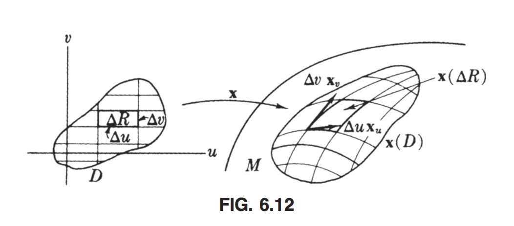
Under the map, it gets distorted into a rectangle with sides $x_u \Delta u$ and $x_v \Delta v$. So, to find the length of the parallelogram, we take the cross product and arrive at $\vert x_u \times x_v \vert \Delta u \Delta v \approx \sqrt{EG - F^2}dudv$. Thus, we define something like an area by integrating this quantity. There’s one small problem: patches have open domains, and integrals are defined for closed and bounded sets. So we define:
Definition: The interior $R^o$ of a rectangle $[a,b]\times [c,d]$ is the open set $(a,b) \times (c,d)$. A two-cell $x:R\rightarrow M$ is called patchlike if the mapping $x:R^o \rightarrow M$ is a patch in $M$.
The function $\sqrt{EG-F^2}$ is bounded in a rectangle, so the area is well-defined and finite. Note that a patchlike segment is not necessarily one-to-one. To define something similar for a more complex region, we add up the areas of a bunch of smaller regions.
Definition: A paving of a region $\mathcal{P}$ in a surface $M$ is a finite number of patchlike 2-segments $x_1, x_2,…x_k$ whose images fill $M$ in such a way that each point of $M$ is in at most one set $x_i(R_i^o)$.
Not all regions are pavable, but it turns out that an entire compact surface is pavable. To find its area, we sum together the area of all its regions.
To get a more rigorous definition in terms of differential forms, we first remember how we defined the integration of a $2$-form $\mu$. We defined:
$$\begin{aligned} \int \int _x \mu = \int \int_R \mu(x_u, x_v) dudv \end{aligned}$$
So in particular, we want to pick a $\mu(x_u, x_v) = \sqrt{EG-F^2}$. We now define such a form.
Definition: An area form on a surface $M$ is a differentiable $2$-form $\mu$ so that its value on any pair of tangent vectors is:
$$\begin{aligned} \mu(v,w) = \pm \vert v\times w \vert \end{aligned}$$
Due to the linearity of forms, equivalently $\mu(E_1, E_2) = \pm 1$ for every frame $E_1, E_2$ on $M$. The sign ambiguity cannot be avoided if we want to keep, for example, Stokes’ Theorem.
Lemma
A surface $M$ has an area form iff it is orientable. On a connected orientable surface, there are precisely two area forms, denoted $\pm dM$.
First, we know that a surface is orientable iff there is a non-vanishing $2$-form on it. So if $M$ has an area form, it is orientable. Given an orientable surface with a unit normal $U$, we can construct its area form:
$$\begin{aligned} dM(v,w) = \pm U\cdot v\times w \end{aligned}$$
To orient a surface, we pick a unit normal. Let $x$ be a patchlike segment, then we can then define:
$$\begin{aligned} \int \int_x dM = \int \int_R dM(x_u, x_v)dudv \end{aligned}$$
There are three cases here depending on the sign of $dM$.
- If $dM(x_u, x_v)$ is positive, we say $x$ is positively oriented; $dM = \sqrt{EG-F^2}$
- If $dM(x_u, x_v)$ is negative, we say $x$ is negatively oriented; $dM = -\sqrt{EG-F^2}$
To find the area of a pavable region $\mathcal{P}$, we must use a paving that is positively oriented (each of its patches is positively oriented). Then we can construct the area by simply summing the integrals over each patchlike segment.
Definition: Let $v$ be a $2$-form on a pavable oriented region $\mathcal{P}$ in a surface. Then, the integral of $v$ over $\mathcal{P}$ is defined:
$$\begin{aligned} \int \int_{\mathcal{P}} v = \sum\limits_i \int \int_{x_i} v \end{aligned}$$
Where $x_1,x_2,…x_k$ is a positively oriented paving of $\mathcal{P}$.
Definition: Let $f$ be a continuous function on a pavable region $\mathcal{P}$, then we define its integral over $\mathcal{P}$ to be:
$$\begin{aligned} \int \int_{\mathcal{P}} f dM \end{aligned}$$
We can rigorously define the integration of any strictly positive function on an arbitrary region by taking the least upper bound of all of its integrals over all pavable regions.
Total Curvature
We define another interesting invariant of a surface, its total curvature.
Definition: Let $K$ be the Gaussian curvature of a compact surface $M$ oriented by an area form $dM$. Then we define the total Gaussian curvature of $M$ as the integral:
$$\begin{aligned} \int \int_{M} K dM \end{aligned}$$
Definition: Let $M,N$ be surfaces oriented by area forms $dM, dN$. Then the Jacobian of the mapping $F:M\rightarrow N$ is the real-valued function $J_F$ so that:
$$\begin{aligned} F^\star(dN) = J_FdM \end{aligned}$$
So essentially, if we pull back an area form on $N$, we want to quantify by how much we shrink to get an area form on $M$:
$$\begin{aligned} J_F dM(v,w) = F^\star(dN)(v,w) = dN(F_\star(v), F_\star(w)) \end{aligned}$$
In particular, this means that $F$ is regular iff $J_F$ is nonzero at a point. The above equation also sufficiently motivates the following definitions:
Definition: If $J_F(p) > 0$, $F$ is orientation preserving at $p$. If $J_F(p) < 0$, it is orientation reversing.
This also motivates a new way of calculating a signed area:
Definition: Let $M,N$ be surfaces with a mapping $F:M\rightarrow N$. Then we define the algebraic area of $F(M)$ to be:
$$\begin{aligned} \int \int_M J_F dM = \int \int_M F^\star(dN) \end{aligned}$$
If $F$ switches orientation on a region, then that region’s area makes a negative contribution, and similarly for preserving orientations.
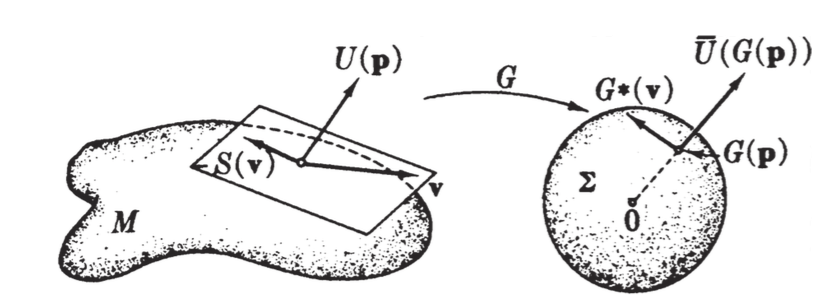
In particular, we look at the Gauss map, which sends each point on a surface to the corresponding unit normal on the unit sphere. From the geometry of a sphere (the unit normal is always pointing outwards), we know that the unit normal $\bar{U}(G(p))$ on the sphere is parallel to to $G(p)$, and thus to $U(p)$ on the original surface itself.
Theorem
The Gaussian curvature $K$ of an oriented surface $M$ is the Jacobian of its Gauss map.
First, note that:
$$\begin{aligned} -S(v) &= \sum v[g_i] U_i(p) \\ G_\star(v) &= \sum v[g_i] U_i(G(p)) \end{aligned}$$
And indeed this means that these two vectors are parallel.
To prove this theorem, we must show the equivalence of the 2-forms: $KdM$ and $G^\star(d\sum)$, where $\sum$ is the unit shere $S^2$. As always, we test this out by applying both forms to the (linearly independent) pair $(v,w)$.
$$\begin{aligned} KdM(v,w) &= K(p)[U(p)\cdot v \times w] \\ &= U(p)\cdot S(v) \times S(w) \end{aligned}$$
To prove that last equality, simply write the matrix of $S$ with respect to the basis $v,w$, take the cross product of an arbitrary pair $(av+bw, cv+dw)$, and note that the result is $\det S v \times w$.
On the other hand, for $G^\star(d\sum)$:
$$\begin{aligned} G^\star(d\sum) = d\sum(G_\star(v), G_\star(w)) = \bar{U}(G(p))\cdot G_\star(v) \times G_\star(w) \end{aligned}$$
First, we noted earlier that $U(p)$ and $\bar{U}(G(p))$ are parallel. Furthermore, $G_\star(v)$ and $-S(v)$ are parallel and the minus signs cancel. So indeed the triple products above are equal.
Corollary
The total Gaussian curvature of an oriented surface $M$ is precisely the algebraic area of the image of its Gauss map $G:M \rightarrow S^2$.
This follows from the earlier theorem simply by integrating over $M$.
Corollary
Let $\mathcal{R}$ be an oriented region in $M$ on which:
- The Gauss map is one-to-one
- $K$ does not change sign
Then the total curvature of $\mathcal{R}$ is, up to a sign, the area of $\mathcal{R}$; the sign is determined by the sign of $K$.
Evidently, this also means that the total curvature is bounded by the area of $\sum$, which is $4\pi$.
On an oriented surface, we can define rotation rigorously as well.
Definition: On an oriented surface, the rotation operator is $J(v) = U \times v$.
This operator rotates tangent vectors by 90 degrees counterclockwise.
Definition: Let $v,w$ be unit tangent vectors at a point $p$ on an an oriented surface $M$. A number $\varphi$ is called an oriented angle from $v$ to $w$ if:
$$\begin{aligned} w = \cos \varphi v + \sin \varphi J(v) \end{aligned}$$
So indeed, an oriented angle measures rotation in the (well-defined) plane determined by $v$ and $J(v)$.
Lemma
Let $\alpha$ be a curve on an oriented surface $M$. If $V,W$ are nonvanishing tangent vector fields on $\alpha$, then there is a differentiable function $\varphi$ on $I$ such that $\varphi$ is the oriented angle between $V(t)$ and $W(t)$.
WLOG, we turn $V$ and $W$ into unit frame fields and define the frame field $V, J(V)$ on $\alpha$. By orthonormal expansion, we can define $W = fV + gJ(V)$. And finally, since $W$ is of unit length, we can define $f=\cos \theta$ and $g = \sin \theta$. $\varphi$ is then called an angle function from $V$ to $W$.
Indeed, on an oriented surface, if we pick $dM$ on positively oriented patches, with positively oriented frame fields, then we have $dM = \theta_1 \wedge \theta_2$.
In particular, given any nonvanishing vector field $V$ on $M$, by the above discussion we can generate a positively oriented frame field. Namely, we take $V, J(V)$ and make them unit length; the resulting frame $E_1, E_2$ is called the associated frame field of $V$.
Congruence of Surfaces
Finally, we get to the moment we’ve been waiting for: establishing congruence of surfaces. We assume for simplicity we’re working with connected, orientable surfaces.
Definition: Two surfaces are congruent if there is an isometry that carries one surface directly onto the other.
Theorem
If $F$ is a Euclidean isometry such that $F(M) = \bar{M}$, then its restriction to $M$ is an isometry of surfaces, and $F$ preserves shape operators, i.e.:
$$\begin{aligned} F_\star(S(v)) = \bar{S}(F_\star(v)) \end{aligned}$$
The first part of this theorem is fairly obvious. The restriction of $F_\star$ should still preserve dot products of tangent vectors, and the restriction of $F$ is by hypothesis one-to-one and onto, and therefore we have an isometry.
We look at the shape operators. Let $U$ be a unit normal in $M$. Since $F_\star$ preserves dot products and therefore orthogonality, $F_\star(U(p))$ is indeed orthogonal to all the tangent vectors at $F(p)$. Thus:
$$\begin{aligned} F_\star(U(p)) = \bar{U}(F(p)) \end{aligned}$$
Where $\bar{U}$ is one of the two unit normals on $\bar{M}$. So we define the two shape operators $S$ derived from $U$ and $\bar{S}$ defined from $\bar{U}$. So we pick a curve $\alpha$ with initial velocity $v$, and map it to $F(\alpha)$, a curve with initial velocity $F_\star(v)$. But we know that the tangent map of an isometry preserves velocities, so:
$$\begin{aligned} F_\star(S(v)) = -F_\star(U') = -[F_\star(U)]' = -\bar{U}' = \bar{S}(F_\star(v)) \end{aligned}$$
And indeed this is well-defined since $v$ and $S(v)$ both lie in the tangent space of $M$.
So we know that by definition, congruent surfaces are isometric. But not all isometric surfaces are congruent. To make the converse relation true, we need to talk about the shape operator. Just as before, we defined congruence by looking at $\kappa$ and $\tau$ for curves, we define congruence for surfaces by looking at the shape operator.
To prove this statement, we first prove a lemma about the congruence of curves theorem, which is instrumental to this generalization.
Lemma
Let $\alpha, \beta$ be two curves defined on the same interval with frame fields $E_1, E_2, E_3$ and $F_1, F_2, F_3$ respectively. For any $t_0 \in I$, if $F$ is the unique Euclidean isometry that sends each $E_i(t_0)$ to $F_i(t_0)$, or equivalently if:
- $\alpha’ \cdot E_i = \beta’ \cdot F_i$
- $E_i’ \cdot E_j = F_i’ \cdot F_j$
Then the two curves are congruent, with $F(\alpha) = \beta$.
We won’t consider the full proof here but the main takeaway is this: if you have two curves for which the velocities have the same expansion (relative to the respective frames) and the derivatives of the frames have the same expansion (relative to the respective frames), then indeed the two curves are congruent.
Theorem
Let $M$ and $\bar{M}$ be oriented surfaces in $\mathbb{R}^3$, and let $F:M\rightarrow \bar{M}$ be an isometry of oriented surfaces between them, such that the shape operators are preserved, i.e.:
$$\begin{aligned} F_\star(S(v)) = \bar{S}(F_\star(v)) \end{aligned}$$
Then, $M$ and $\bar{M}$ are congruent; there is a Euclidean isometry whose restriction is precisely $F$.
I’ll just proceed with the sketch of a proof here. First, we take the unique Euclidean isometry which pushes forward a tangent frame at $p$ in $M$ to precisely the pushforward of that tangent frame under $F$, and which pushes forward the unit normal $E_3$ at $p$ determining the shape operator of $M$ to the unit normal $\bar{E_3}$ at $F(p)$ determining the shape operator of $\bar{M}$. In other words, if we have a Euclidean isometry whose restriction to $M$ is $F$, then certainly its tangent map agrees with that of $F$. Fix a point $p_0$ and for any point $p$, let $\alpha$ be any curve in $M$ between the two points.
Next, transfer a tangent frame field on $M$ via the isometry $F$ to a tangent frame field on $\bar{M}$, and append the respective unit normals to get adapted frame fields for $M, \bar{M}$.
Finally, we confirm the conditions of our previous lemma using the properties of isometries (they preserve velocities and derivatives). The expansion of $\alpha’$ in the first frame is the same as the expansion of $F(\alpha’)$ in the second frame. Using the pullback of the connection forms as well as the fact that isometries preserve shape operators, we prove that $E_1, E_2$ has the same expansion in $M$ as $\bar{E_1}, \bar{E_2}$. Thus, we have found a Euclidean isometry which restricts to $F$; and indeed, this means every curve in $M$ is congruent to a curve in $\bar{M}$, so we are done.
To draw analogy with the congruence theorem for curves: isometries between (orientable, connected) surfaces function sort of like reparametrizations of unit-speed curves on the same interval. And matching curvatures and torsions loosely correspond to matching shape operators. Putting the two kinds of hypotheses together yields a sufficient condition for congruence.
Download this Page as a PDF:
Note: Images are replaced by captions.
Recent Posts
- A Note on the Variation of Parameters Method | 11/01/17
- Group Theory, Part 3: Direct and Semidirect Products | 10/26/17
- Galois Theory, Part 1: The Fundamental Theorem of Galois Theory | 10/19/17
- Field Theory, Part 2: Splitting Fields; Algebraic Closure | 10/19/17
- Field Theory, Part 1: Basic Theory and Algebraic Extensions | 10/18/17