Differential Geometry Part IV: Calculus on Surfaces
July 12th, 2017
In this section, we discuss calculus on surfaces. Concretely, surfaces in $\mathbb{R}^3$ are comparable to sections of the Euclidean plane $\mathbb{R}^2$; with this correspondence, we can carry over much of the tools from calculus to surfaces (functions, vector fields, differential forms) and consider surfaces regardless of their ambient context.
Surfaces in $\mathbb{R}^3$
Definition: Suppose we have a set of points $M\subset \mathbb{R}^3$. A coordinate patch $x:\ D\subset \mathbb{R}^2 \rightarrow M$ is a one to one, smooth, regular mapping of an open set $D\subset \mathbb{R}^2$ into $\mathbb{R}^n$. A proper patch has a continuous inverse $x^{-1}$; in other words, a proper patch of $M$ is a homemorphism from Euclidean space to a subset of $M$.
What we will do is construct an object as a union of (possibly overlapping) patches. Each mapping is one-to-one with a one-to-one tangent map everywhere, so we’re sure this map is well-defined for our purposes. Now we can define a surface:
Definition: A surface is a $M\subset \mathbb{R}^3$ such that for each point $p\in M$, there is a proper patch from $\mathbb{R}^2$ to a neighborhood of $p$.
An important example is the graph of a differentiable function $f(x,y)$, which is evidently a surface with coordinate patch given by $x(u,v) = (u,v,f(u,v))$. We can extend this idea to prove that level sets are surfaces, given a reasonable criterion.
Theorem
Let $g$ be a differentiable real-valued function on $\mathbb{R}^3$. Let $M= {(x,y,z)\ \vert\ g(x,y,z)=c}$. Then, $M$ is a surface if $dg\ne 0$ anywhere on $m$.
If you think about it, this is kind of a corollary of the Implicit Function Theorem (one of the only two useful theorems you learn in advanced calculus, along with the Inverse Function Theorem). We recall our definition of $dg$, which is a $1$-form:
$$ dg = \frac{\partial g}{\partial x}dx +\frac{\partial g}{\partial y}dy + \frac{\partial g}{\partial z}dz $$
So the criterion that $dg\ne 0$ is equivalent to saying that the gradient of $g$ is not zero anywhere. Let’s pick a point $p=(p_1, p_2, p_3)$, and say WLOG that $g_z \ne 0$. By the implicit function theorem, there is a (unique) differentiable function h so that for all $(u,v)$ in the neighorhood of $(p_1, p_2)$, $g(u,v,h(u,v)) = c$. So for every point, we have constructed a proper patch $x(u,v) = (u,v,h(u,v))$; thus $M$ is a surface.
For example, this means that a sphere is a surface, as are surfaces of revolution.
Definition: Let $x:\ D\rightarrow \mathbb{R}^3$ be a patch. Then at each point $u=(u_0, v_0)$, we define two separate curves $u \rightarrow x(u,v_0)$ and $v \rightarrow x(u_0, v)$. Their respective velocities are called partial velocities and are denoted $x_u$ and $x_v$.
Note that $x_u$ and $x_v$ are tangent vectors applied at a given point. It isn’t hard to see that if our patch is $x = (x_1, x_2, x_3)$, then:
$$ x_u = (\frac{\partial x_1}{\partial u},\frac{\partial x_2}{\partial u},\frac{\partial x_3}{\partial u}) $$
So this operation works very much like partial differentiation. We also define parametrization the usual way:
Definition: A regular mapping $x:\ D:\rightarrow M \subset \mathbb{R}^3$ is called a parametrization of $M$. With our definition of partial velocities from earlier, we can construct an easy test to see if $x$ is a regular mapping. Let $U_1, U_2, U_3$ be the coordinate functions. Then we define the cross product:
$$ x_u \times x_v = \begin{bmatrix} U_1 & U_2 & U_3 \\ \frac{\partial x_1}{\partial u} & \frac{\partial x_2}{\partial u} & \frac{\partial x_3}{\partial u} \\ \frac{\partial x_1}{\partial v} & \frac{\partial x_2}{\partial v} & \frac{\partial x_3}{\partial v} \\ \end{bmatrix}$$
The last two rows of this matrix, notice, are the transpose of the Jacobian matrix. To say that a mapping is regular, then, is to say that its partial velocities are linearly independent, or equivalently that $x_u \times x_v \ne 0$ throughout $D$.
Now that we have defined a surface in multiple ways, we can begin the difficult task of defining differentiation.
Tangent Vectors, Vector Fields, and Directional Derivatives
From here on, we will mirror Part 1 of my notes, defining derivatives, 1-forms, and mappings. A lot of the proofs in this section are tedious and unenlightening, so I’ll try my best to stick to the Cliffs Notes.
Definition: Suppose that $f$ is a real-valued function defined on a surface $M$. Then $f$ is differentiable if $f\circ x:\ D \rightarrow M$ is differentiable for any patch $x$ of $M$.
Definition: Consider a function $F: S\subset \mathbb{R}^n \rightarrow M$. Then $F$ is differentiable if for every patch $x:\ D\rightarrow M$, the function $x^{-1}\circ F$ is differentiable. We must first define $\mathcal{O} = (p\in \mathbb{R}^n \mid F(p) \in x(D))$ so that the composite function is well-defined; then, differentiability of $x^{-1}(F):\ \mathcal{O}\rightarrow \mathbb{R}^3$ is defined in the usual way if $\mathcal{O}$ is an open set.
As a result, we can define coordinate functions of any function $F$ with respect to a patch $x$. For example, look at a curve $\alpha: I \rightarrow M$. Then, $x^{-1}\circ \alpha: I\rightarrow D = (a_1, a_2)$ And so we have:
$$ \alpha = x(a_1, a_2) $$
Since $\alpha$ is differentiable, you can then say that $\alpha_1, \alpha_2$ are differentiable functions. You might already see a problem here, which is that patches can overlap and give us disagreeing coordinate functions. We’ll deal with that in a little bit.
There is a natural equivalence between our two concepts of differentiable maps. If we take a differentiable mapping $F:\ \mathbb{R}^n \rightarrow \mathbb{R}^3$ whose image lies in $M$, then considered as a function on manifolds, it is differentiable (as above). In other words, if the restriction of a mapping onto $M$ is differentiable, then $F$ works smoothly with all patches on $M$.
The proof is basically an exercise in set theory, so I’ll spare you the details which you can read here if you’re curious. Also, I just realized that the term “atlas” is a pun, I guess, because in real life an atlas is a collection of maps, and a chart is a map. Wow. Anyway, it follows that since patches are differentiable mappings, they are differentiable on manifolds (meaning they agree with all other patches). More formally, we state the following corollary.
Corollary
If $x$ and $y$ are overlapping patches for $M$, then $x^{-1}y$ and $y^{-1}\circ x$ are differentiable mappings defined on open sets of $\mathbb{R}^2$.
Indeed, since these composite functions are differentiable, their coordinate functions are differentiable, i.e., there exist unique differentiable functions $\bar u, \bar v$ so that:
$y = x(\bar{u}, \bar{v})$.
With this lemma, we don’t have to check differentiability using all patches, only enough patches to cover $M$, because we can transition between different patches using a smooth map (albeit on a smaller domain). Now that we have differentiation, we’re move on to define tangent vectors.
Definition: Let $p\in M$ be a point on a surface in $\mathbb{R}^3$. Then, a tangent vector $v$ to $\mathbb{R}^3$ at $p$ is tangent to $M$ at $p$ if $v$ is the velocity of some curve in $M$. The set of all such tangent vectors is called the tangent plane of $M$ at $p$, denoted $T_p(M)$.
So we now have a way of constructing tangent spaces of surfaces, where instead we only had the tangent space of $\mathbb{R}^3$. Now let’s prove that a tangent plane is actually a plane (i.e. two dimensional).
Lemma
Let $p$ be a point of a surface $M$ in $\mathbb{R}^3$, and let $x$ be a patch so that $x(u_0, v_0) = p$. Then the partial velocities $x_u, x_v$ at $(u_0,v_0)$ form a basis for the tangent plane at $M$.
We get for free that the partial velocities are linearly independent; we must only show that they span the tangent plane. Firstly, as we saw before, $x_u$ and $x_v$ are velocities of curves in $M$ through $p$. Suppose we have another vector $v$ in the tangent plane; then there is some curve $\alpha$ with $\alpha(0)=p$ and $\alpha’(0)=v$.
Let $(a_1,a_2)$ be the Euclidean coordinate functions for $x^{-1}\circ \alpha$. Then $\alpha = x(a_1, a_2)$. But then, by the chain rule:
$$ \alpha' = x_u \frac{da_1}{dt} + x_v \frac{da_2}{dt} $$
Where $x_u,x_v$ are evaluated at $p$. So we are done. It is not hard to prove that every linear combination of $x_u, x_v$ is a tangent vector as well.
Now that we have tangent vectors, we define vector fields straightforwardly.
Definition: A Euclidean vector field $Z$ on a surface $M\subset \mathbb{R}^3$ is a function that assigns to each $p\in M$ at tangent vector $Z(p)$ to $\mathbb{R}^3$ at $p$.
Note that vector fields do not necessarily give us vectors in the tangent plane. Such a vector field is instead called a tangent vector field. This is important because we can define things like a normal vector field. I will leave out the simple proof that for a level set which is a surface, the gradient vector field is a non-vanishing normal vector field. Finally, we are ready to describe derivatives, or how tangent vectors are applied to functions at points.
Definition: Let $v$ be a tangent vector to $M$ at $p$, and let $f$ be a differentiable real-valued function on $M$. We define the derivative $v[f]$ as $\frac{d}{dt}(f\alpha (t))$ at $t=0$ for any curve $\alpha$ with $\alpha’(0)=v$ and $\alpha(0)=p$.
This definition is pretty much the same as the one we had earlier for the directional derivative, except instead of taking a derivative along a line, we’re taking a derivative along a curve through $M$ at $p$. By the chain rule, you can see that the directional derivative does not depend on which curve $\alpha$ we pick. Finally, the usual properties of linearity and the Leibniz rule hold.
Differential Forms on a Surface
Forms on a manifold (as we will see later, a generalization of a surface) can tell us quite a bit about its geometry, as we will soon see. Our definitions normally.
- A $0$-form is a differentiable real-valued function on $M$.
- A $1$-form is a real-valued linear function on tangent vectors to $M$ at $p$.
- A $2$-form is a real-valued linear function on pairs of tangent vectors to $M$ at $p$.
A $1$-form can be evaluated as before on a vector field $V$, and $2$-forms on pairs of vector fields $V,W$.
More concretely, a $2$-form $\eta(v,w)$ is linear in both its arguments and antisymmetric, i.e. $\eta(v,w) = -\eta(w,v)$. As a result, we can determine the value of a $2$-form just based on its evaluation on two linearly independent tangent vectors $v$ and $w$. In fact, the result looks like the determinant:
$$ \eta(av+bw, cv+dw) = \det\begin{bmatrix} a & b \\ c & d\end{bmatrix} \eta(v,w) $$
The only thing we’re missing is a suitable definition for the wedge product of two $1$-forms on a surface. We define:
Definition: If $\phi$ and $\psi$ are $1$-forms on $M$, then the wedge product $\phi \wedge \psi$ is the $2$-form on $M$ such that:
$$ (\phi \wedge \psi)(v,w) = \phi(v)\psi(w) - \phi(w)\psi(v) $$
So we have the usual anticommutative property from our definition. In general, a wedge product of a $p$-form $\xi$ and a $q$-form $\eta$ has the law: $\xi \wedge \eta = (-1)^{pq} \eta \wedge \xi$. So on a surface, a minus sign only occurs when computing the wedge product of two $1$-forms.
Now we move on to the exterior derivatives of forms on a surface. As before, we define the exterior derivative of a $0$-form $f$ to be the $1$-form $df$ so that $df(v) = v[f]$; we already defined directional derivatives so this makes sense. The only missing ingredient is the exterior derivative of a $1$-form (which ought to be a $2$-form).
Definition: Let $\phi$ be a $1$-form on a surface $M$. Then the exterior derivative $d\phi$ is the $2$-form such that for any patch $x$ in $M$:
$$ d\phi(x_u, x_v) = \frac{\partial}{\partial u}(\phi(x_v)) - \frac{\partial}{\partial v}(\phi(x_u)) $$
You can check that this is indeed a $2$-form. The issue here is that patches can overlap. We denote the above definition as $d_x\phi$. So our goal is to show when two patches $x$ and $y$ overlap at a point, then $d_x\phi = d_y\phi$.
Lemma
We claim that definition above for the exterior derivative is well-defined, i.e. for any two overlapping patches $x$ and $y$, $d_x\phi = d_y\phi$ on their overlap.
Consider any two linearly independent tangent vectors $y_u$ and $y_v$. From the earlier discussion, we know that $d_x\phi(y_u, y_v)$ completely determines $d\phi$. We also know from earlier that we can find coordinate functions for $y$ with respect to $x$, i.e. $y = x(\bar{u}, \bar{v})$. But then by the chain rule:
$$\begin{aligned} y_u &= \frac{\partial \overline{u}}{\partial u}x_u + \frac{\partial \overline{v}}{\partial u}x_v \\ y_v &= \frac{\partial \overline{u}}{\partial v}x_u + \frac{\partial \overline{v}}{\partial v}x_v \end{aligned}$$
But now we can use the determinant fact from earlier to rewrite:
$$ d_x\phi(y_u, y_v) = \det\begin{bmatrix} \frac{\partial \overline{u}}{\partial u} & \frac{\partial \overline{v}}{\partial u} \\ \frac{\partial \overline{u}}{\partial v} & \frac{\partial \overline{v}}{\partial v}\end{bmatrix} d_x\phi(x_u, x_v) $$
We can regard the matrix above as a sort of a Jacobian matrix (of the coordinate functions of $y$), or at least its transpose. Regardless, we denote $J$ to be the determinant of that matrix and write succinctly:
$$ d_x\phi(y_u, y_v) = J d_x\phi(x_u, x_v) $$
The rest of the proof proceeds by using the chain rule, but it is a tedious proof which I will omit here. Perhaps a more enlightening (and succinct) form of writing the exterior derivative of $1$-forms on a surface is:
$$ d\phi(V, W) = V[\phi(W)] - W[\phi[V]] $$
Where $\phi(W)$ is a function since $\phi$ is a one form, and so we can take directional derivatives. You can check that the two definitions are equivalent. The second definition shows us linearity and anti-commutativity far more clearly. Next we prove another property of exterior derivatives, which is that $d^2 = 0$. We only need to check this for $0$-forms on a surface.
Theorem
If $f$ is a real-valued function on $M$, then $d(df)=0$.
First, we write $\psi = df$; we claim that $d\psi=0$. We have:
$$\begin{aligned} \psi(x_u) &= df(x_u) = x_u[f] = \frac{\partial}{\partial u}f(x) \\ \psi(x_v) &= df(x_v) = x_v[f] = \frac{\partial}{\partial v}f(x) \\ \end{aligned}$$
By the equality of mixed partial derivatives, you can check that the terms in $d\psi$ cancel.
Let’s look at an example and examine differential forms on the plane.
Differential Forms on the Plane
Define $u_i$ to be the natural coordinate functions, $U_i$ the natural frame field (in other words, $du_i$ are the dual forms of $U_i$). Let $f$ be a function on $M$. Then all $1$-forms look like
$$ \phi = f_1 du_1 + f_2 du_2 $$
Where $\phi(U_i) = f_i$. The two forms are:
$$ \eta = gdu_1du_2 $$
Where $g = \eta(U_1, U_2)$. If we define $\psi = g_1u_1 + g_2 u_2$, then we can take the wedge product:
$$\phi \wedge \psi = (f_1g_2 - f_2g_1)du_1 du_2$$
We can take the exterior derivative of the $0$-form $f$:
$$ df = \frac{\partial f}{\partial u_1}du_1 + \frac{\partial f}{\partial u_2}du_2 $$
And the exterior derivative of the $1$-form $\phi$ is:
$$ d\phi = (\frac{\partial f_2}{\partial u_1}- \frac{\partial f_1}{\partial u_2})du_1 du_2 $$
We end this section with one last definition.
Definition: A differential form $\phi$ is closed if $d\phi=0$. A differential form $\phi$ is exact if $\phi = d\xi$ for some $\xi$.
You may recognize the exact differential forms from differential equations; exact differential equations can be easily solved using Stokes Theorem.
Mappings of Surfaces
We now define mappings between surfaces in a straightforward generalization of the ideas we’ve seen so far for mappings.
Definition: A function $F:M\rightarrow N$ between surfaces is differentiable if for each patch $x$ in $M$ and $y$ in $N$, the composite function $y^{-1}\circ F \circ x: D\rightarrow D’$ is differentiable. This is called a mapping between surfaces.
As before, we don’t need to check every pair of patches, but only enough patches to cover the two surfaces since we can transition smoothly between patches.
We can prove, for example, that the stereographic projection is a differentiable map between surfaces. Now we define the tangent map.
Definition: Let $F:M\rightarrow N$ be a mapping between surfaces. Then, the tangent map $F_\star$ assigns to each tangent vector $v$ to $M$ at $p$ a tangent vector $F_\star(v)$ to $N$ at $F(p)$. We define $F_\star(v)$ as follows: if $v$ is the initial velocity of a curve $\alpha$ in $M$, then $F_\star(v)$ is the initial velocity of the curve $F(\alpha)$ in $N$.
It is maybe not evident, but $F_\star$ is a linear map between $T_p(M)$ and $T_{F(p)} N$. By construction, this map preserves velocities of curves; notably, partial velocities get sent to partial velocities. We can rewrite succinctly for any curve $\alpha$ through $p \in M$:
$$ F_\star (\alpha'(0)) = (F\circ \alpha)'(0) $$
We define a mapping to be regular if its tangent map (a square matrix) is one-to-one at each point; equivalently, if $F_\star$ is a linear isomorphism (invertible square matrix). A mapping with an inverse is called a diffeomorphism. This leads us to a special case of the inverse function theorem:
Theorem (Inverse Function Theorem)
Let $F:M\rightarrow N$ be a mapping of surfaces such that $F_{\star,p}$ is a linear isomorphism for some $p\in M$. Then there is a neighborhood of $p$ so that the restriction of $F$ to that neighborhood yields a diffeomorphism onto a neighborhood of $F(p)$ in $N$.
We also have that a regular one-to-one mapping $F$ of $M$ onto $N$ is a diffeomorphism, from definitions. Essentially, diffeomorphic objects are the same up to a smooth transformation.
Now, since mappings of surfaces map tangent vectors to tangent vectors in a well-defined way, we can imagine differential forms being easily transferrable between surfaces by a composition of functions. More concretely:
Definition: Let $F:M\rightarrow N$ be a mapping of surfaces, and $\phi$ a $1$-form on $N$. Then, define $F^\star \phi$ to be the $1$-form on $M$ so that:
$$ (F^\star \phi) (v) = \phi(F_\star v) $$
for all tangent vectors $v$ to $M$.
Remark
It may be useful to consider the terms “pushforward” and “pullback”. A “pushforward”, or differential, is the tangent map we saw earlier. It pushes “forward” because it sends tangent vectors in $M$ to tangent vectors in $N$.
On the other hand, we also have $F^\star$, which pulls “back” because given a mapping $F$ from $M$ to $N$, it pulls back a differential form on $N$ to a differential form on $M$, thus moving “backwards” through the map. I’ll be using these terms from now on.
We can do the same for two forms:
Definition: Let $F:M\rightarrow N$ be a mapping of surfaces, and $\eta$ a $2$-form on $N$. Then, define $F_\star \eta$ to be the $2$-form on $M$ so that:
$$ (F^\star \eta) (v,w) = \eta(F^\star(v), F^\star(w)) $$
We will also denote $F^\star(f)$ = $f(F)$ for $0$-forms or functions on $N$, for consistency; $F^\star$ denotes a pullback, which make sense here as we are pulling back a function on $N$ to a function on $M$. We finally end up with these elegant formulas for forms:
Theorem
Let $F:M\rightarrow N$ be a mapping of surfaces, and $\eta$ and $\xi$ are forms on $N$. Then we have:
- $F^\star (\eta + \xi) = F^\star(\eta) + F^\star(\xi)$.
- $F^\star (\eta \wedge \xi) = F^\star(\eta) \wedge F^\star(\xi)$.
- $F^\star (d\xi) = d(F^\star \xi)$
The first two statements are pretty straightforward computations. The last one has a proof that’s a little bit long, but not too important to the general understanding of the ideas, so I will omit it.
Integration on Surfaces
Recall how we defined calculus in Euclidean space; we integrate, for example, with respect to $1$-forms $dx$ and $dy$. But now that we have differential forms on surfaces, we can pull them back to Euclidean space and then integrate there. Thus we can formally define integration on surfaces.
For example, consider a curve on a surface $\alpha: I \rightarrow M$. Then what is the pullback of a $1$-form on $M$? It is a $1$-form on $\mathbb{R}$, so it is of the form $f(t)dt$ for some $f$. To find the coefficients of the $i$th dual form, we evaluate $E_i$; in this case we only need to evaluate $\alpha^{\star} \phi(U_i)$. So we have:
$$ (\alpha^{\star} \phi)(U_1) = \phi(\alpha_\star(U_1)) $$
Recall how we defined the tangent map:
$$ F_\star (v) = \sum v[f_i]U_i $$
And in this case:
$$ \alpha_\star (U_1) = U_1[\alpha] = \alpha'(t) $$
So for any $1$-form $\phi$ on $M$, and a curve $\alpha(t)$, we have a pullback $\alpha^\star = \phi(\alpha’(t))dt$. This is a fairly flexible result and we can do a lot with it.
Definition: Let $\phi$ be a $1$-form on $M$ and let $\alpha:[a,b]\rightarrow M$ be a curve in $M$. Then we define the integral of $\phi$ over $\alpha$ as follows:
$$ \int_\alpha \phi = \int_{[a,b]} \alpha^\star(\phi) = \int_a^b \phi(\alpha'(t))dt $$
This should look a lot like the definition of a line integral. And indeed, we can, for example calculate work. Suppose we have some vector field $V$, representing a force field, and consider the dual form $\phi$ to $V$, defined analogously to how we defined dual forms for frame fields in Part II. So we define $\phi(w) = w\cdot V$ at each point. Then, we can elegantly write the formula for work as a line integral:
$$ W = \int_\alpha V(\alpha(t))\cdot \alpha'(t)dt = \int_\alpha \phi(\alpha'(t))dt = \int_\alpha \phi $$
What if $\phi$ is an exact form, i.e. $\phi = df$ for some $0$-form $f$? We get the corresponding generalization of the fundamental theorem of calculus.
Theorem
Let $f$ be a function on $M$, and let $\alpha$ be a curve where $\alpha(a)=p, \alpha(b)=q$. Then we claim that:
$$ \int_\alpha df = f(q) - f(p) $$
As a corollary, this means that exact forms (related in physics to conservative vector fields) are independent of path, and vanish on closed paths. The proof comes from definitions:
$$ \int_\alpha df = \int_a^b df(\alpha')dt $$
But we earlier defined the action of $1$-forms on surfaces:
$$ df(\alpha') = \alpha'[f] = \frac{d}{dt}(f\circ \alpha) $$
Where we omitted here the point of application determined by $t$. Returning to our integral, we have:
$$ \int_\alpha df = \frac{d}{dt}(f\circ \alpha(t)) dt = f(\alpha(b)) - f(\alpha(a)) = f(q) - f(p) $$
And we get the result by the fundamental theorem of calculus.
The amazing thing is that we can do something very similar if we pull back a $2$-form $\xi$ on $M$. Again, we know that the pullback will be of the form $h(u,v)dudv$, and we can compute $h$ explicitly by calculating $h = x^\star \xi (U_1, U_2)$. But we have from our definitions:
$$ h = (x^\star \eta)(U_1, U_2) = (\eta)(x_\star (U_1), x_\star (U_2)) $$
We check that $x_\star(U_1) = \sum U_1[x_j] \bar{U_j} = x_u$, and proceed similarly for the other term; so our computation above simplifies to:
$$ h = (x^\star \eta)(U_1, U_2) = \eta (x_u, x_v) $$
Now that we can pull back $2$-forms, we can accordingly define double integrals over surfaces.
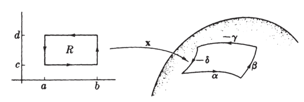
Definition: Let $\eta$ be a $2$-form on $M$, and let $x:R\rightarrow M$ be a map from a rectangle $[a,b]\times[c,d]$ in the plane into $M$. Then the integral of $\eta$ over $x$ is defined as:
$$ \int \int _x \eta = \int \int _R x^\star \eta = \int_a^b \int_c^d \eta(x_u, x_v)dudv $$
The corresponding “conservation” theorem, wherein we compute the integral of an exact $2$-form on $M$, gives us none other than Stokes’ Theorem.
Theorem: Stokes’ Theorem
We will compute the integral of a $2$-form $\eta = d\phi$ over $x$ as above. First, we define a boundary $\partial x$ for $x$, which is a closed curve. We do this by defining its four sections:
- $\alpha(u) = x(u,c)$
- $\beta(v) = x(b,v)$
- $\gamma(u) = x(u,d)$
- $\delta(v) = x(a,v)$
Then we define the boundary as the counterclockwise traversal of these four segments, i.e. $\delta x = \alpha + \beta - (\gamma + \delta)$.
Now we can state the Stokes’ Theorem in full:
$$ \int \int _x d \eta = \int_{\partial x} \phi $$
Proof
We first apply our definition above to rearrange the integral on the left hand side:
$$ \int \int _x d\phi = \int_a^b \int_c^d d \phi(x_u, x_v)dudv $$
And from our definition of the exterior derivative of a $1$-form earlier, we can rewrite:
$$ \int \int_R d \phi(x_u, x_v)\ dudv =\int \int_R \left[\frac{\partial}{\partial u}\phi(x_v) - \frac{\partial}{\partial v}\phi(x_u)\right]\ dudv $$
For convenience sake, we write $f = \phi(x_u)$ and $g=\phi(x_v)$, to arrive at:
$$ \int \int_R d \phi(x_u, x_v)\ dudv =\int \int_R \frac{\partial g}{\partial u}\ du dv - \int \int_R \frac{\partial f}{\partial v}\ dudv $$
Let’s take a look at the integral on the left hand side. We treat it as an interated integral, i.e. define $I(v) = \int_a^b \frac{\partial g}{\partial u}\ dudv$:
$$ \int \int_R \frac{\partial g}{\partial u}\ du dv = \int_c^d I(v) dv $$
Now note that for a given fixed value of $v$, the integrand of $I(v)$ is not a partial derivative but just a derivative. We then apply the fundamental theorem of calculus to get:
$$\begin{aligned} I(v) &= \int_a^b \frac{dg}{du}du = g(b,v) - g(a,v) \\ \int \int_R \frac{\partial g}{\partial u}dudv &= \int_c^d g(b,v)dv - \int_c^d g(a,v)dv \end{aligned}$$
Now, we look at the left integral, remembering that we defined earlier $g=\phi(x_v)$. Using our boundary from earlier, we have that $x_v(b,v) = \beta’(v)$. So finally we write:
$$ \int_c^d g(b,v)dv = \int_c^d \phi(\beta'(v)) dv = \int_\beta \phi $$
Repeating this argument for the other integral above, we have:
$$ \int \int_R \frac{\partial g}{\partial u}dudv = \left( \int_\beta \phi - \int_\delta \phi \right) $$
Continuing onwards, we finally arrive at:
$$ \int \int_x d\phi = \left(\int_\beta \phi - \int_\delta \phi \right) - \left(\int_\gamma \phi - \int_\delta \alpha \right) = \int_{\partial x} \phi $$
And we are done. We also note that reparametrizations can be orientation-preserving or orienation reversing, which affect the line integral by a sign.
Topological Properties of Surfaces
I will assume here a basic knowledge of concepts in topology such as connectedness and compactness. We’ll look at how these properties can be defined on a surface.
Definition: A surface is connected if for each $p,q \in M$, there is a curve from $p$ to $q$ in $M$.
Lemma
A surface $M$ is compact iff it can be covered by the images of a finite number of rectangles in $M$.
First, we prove the backwards direction. Suppose $M$ is compact. For each $p\in M$, $p$ lies in the image of some rectangle under a patch $x$. A finite number of such patches covers $M$, since $M$ is compact; therefore the number of corresponding rectangles is finite.
Conversely, assume that $M$ is covered by the images of a finite number of rectangles.
We first prove a lemma, that the image of a rectangle under a patch $x$ is compact. Since $x$ is differentiable, we assume it can be extended to an open set containing the rectangle.
Now, let $(U_\alpha)$ be an open covering of $M$,and $r\in D$ be a point in the rectangle. Then $x(r) \in U_r$ for some $U_r \in (U_\alpha)$. Since $x$ is continuous, the preimage of $U_r$ is a neighborhood $N_r$ in the rectangle. For all $r$, these neighborhoods form an open covering of the rectangle. Since there are finitely many $N_r$, there are finitely many $U_r$; thus, we have constructed a finite covering of $x(R)$.
Returning to the original problem, assume that $M$ is covered by the images of a finite number of rectangles. Suppose that we have some open covering for $M$. We just showed that the image of each rectangle is covered by a finite subcovering; therefore, taking a finite union of finite sets, we arrive at a finite subcovering for $M$.
Lemma
A continuous function on a compact region in a surface $M$ takes on a maximum somewhere in the region.
This lemma follows straightforwardly from the similar theorem that a function in a compact region in Euclidean space (a rectangle) attains a maximum.
This can show us that many objects are not compact. For example, a cylinder is not compact since the coordinate $z$ is unbounded. Loosely, you expect a compact object to be closed with a smooth boundary.
Definition: A surface $M$ is orientable if there exists a differentiable $2$-form $\mu$ on $M$ which does not vanish on $M$.
This definition makes a little more sense if we connect it to unit normal vector fields.
Proposition
A surface $M$ in $\mathbb{R}^3$ is orientable iff there is a unit vector field $U$ on $M$. If $M$ is connected, then $\pm U$ are the only two unit normal vector fields.
Proof
First, we prove the backwards direction. Say that there is a unit normal vector field $U$ on $M$. Then we can define:
$$ \eta(v,w) = U \cdot (v\times w) $$
It is clear that this is a $2$-form, since the determinant is linear in its rows, and the cross product is anti-symmetric. The $2$-form is determined by its value on a linearly independent pair of vectors, in which case the three vectors $U,v,w$ are linearly independent, and so the triple product is non-zero.
Conversely, suppose that $M$ is orientable and there is a non-vanishing $2$-form $\mu$. Then define the following vector field:
$$ Z(p) = \frac{v \times w}{\mu(v,w)} $$
Where $v,w$ are any two linearly independent tangent vectors. Since they are two tangent vectors, their cross product is a normal vector; if you check its magnitude, it is the determinant of the coordinates of $v,w$, which is a multiple of $mu(v,w)$. So this vector field is normal to each tangent plane, does not vanish and does not depend on the choice of $v,w$. To make it a unit normal vector field, all we have to do is divide by the magnitude.
On a connected surface, a non-vanishing differential function cannot change sign (intermediate value theorem), so that up to sign, there is only one unit normal vector field.
For example, level sets have a unit normal vector field (the gradient), so they are all orientable. Similarly, parametrizations are orientable.
Definition: A closed curve $\alpha$ in $M$ is homotopic to a constant if there is a rectangle $R$ and a patch $x: R\rightarrow M$, called a homotopy, defined on $[a,b]\times[0,1]$, such that $x(u,0) = \alpha(u)$ and the other three edge curves $x(u,1), x(b,v), x(u,1) = \alpha(a) = \alpha(b) = p$ are constant.
Intuitively, a homotopy is a continuous deformation. This motivates our definition:
Definition: A surface $M$ is simply connected if it is connected and every loop in $M$ is homotopic to a constant.
This means, intuitively, that there are no “holes”; each loop in $M$ can be shrunk down to a single point. We can come up with a fairly easy test for simple connectedness:
Lemma
Let $\phi$ be a closed $1$-form on $M$. If a loop $\alpha$ is homotopic to a constant, then $\int_\alpha \phi = 0$.
The proof is straightforward. $d\phi=0$ by definition. By Stokes’ Theorem, $\int_{\partial x} \phi = 0$ for any boundary $\partial x$. In particular, there is a boundary on which three edges are constant, so that $\int_{\partial x} \phi = \int_\alpha \phi = 0$.
Next, we consider that earlier we defined exact forms such that every exact form is closed (since $d^2=0$). But under what conditions is a closed form exact? Well, turns out, on any simply connected surface, this is true for $1$-forms.
Lemma (Poincaré)
This nice lemma says that on a simply connected surface, every closed $1$-form is exact; so that if $d\phi = 0$, then $\phi = df$ for some $f$.
Proof
First, we show that the integral of a closed $1$-form is path independent on a simply connected surface. Suppose we have two curves $\alpha$ and $\beta$ from $p$ to $q$. Then $\alpha - \beta$ is a closed loop. Every loop on a simply connected surface is homotopic to a constant. Thus, by our lemma, $\int_{\alpha - \beta} \phi = 0$, or equivalently $\int_\alpha \phi = \int_\beta \phi$.
Now, suppose that $\phi$ is a $1$-form on a simply connected surface. We define $f(p) = \int_\delta \phi$, where $\delta$ is any curve from a fixed point $p_0$ to $p$. From earlier, we know that $f$ is well-defined everywhere. We claim then, that $df = \phi$, or in other words that $df(v) = \phi(v)$ for every tangent vector at $p$.
Let $\alpha: [a,b] \rightarrow M$ be any curve with initial velocity $\alpha’(a)=v$ and initial position $\alpha(a) = p$. Then we can append this curve to $\delta$ to obtain a curve from $p_0$ to $\alpha(t)$. Let’s call this curve $\gamma$. By the definition of $f$:
$$ f(\alpha(t)) = \int_\gamma \phi = f(p) + \int_a^t \phi(\alpha'(u))du $$
Taking the derivative and applying the fundamental theorem of calculus, we have $\alpha’[f] = (f\circ \alpha)’(t) = \phi(\alpha’(t))$. In particular, at $t=0$, we get $v[f] = \phi(v)$. Indeed, $df(v) = \phi(v)$. This construction is more or less what we would expect, and mirrors the proof of the fundamental theorem of calculus.
I leave the last two theorems in this section without proof, as we’ll get to them later.
Theorem
A compact surface in $\mathbb{R}^3$ is orientable. (Corollary of the Jordan Curve Theorem)
Theorem
A simply connected surface is orientable.
Manifolds
Now we will generalize the basic concepts about surfaces to consider examples beyond $\mathbb{R}^3$. First we start with patches. We may have an abstract patch, which is a one-to-one map from $D \subset \mathbb{R}^2$ into the set $M$, which does not necessarily sit inside an ambient Euclidean space. By gluing together abstract patches, we get a manifold.
Definition: A surface is a set $M$ with a collection $\mathcal{P}$ of abstract patches satisfying the following axioms.
- The images of the patches $\mathcal{P}$ cover $M$.
- Patches smoothly overlap. For any patches $x,y\in \mathcal{P}$, the composite functions $x^{-1}y, y^{-1}x$ are differentiable in the Euclidean sense, defined on open sets in $\mathbb{R}^2$.
We also wish to define a topology on the surface. So, for any patch $x$, the image of an open set in $D$ is an open set in $M$, as well as their unions. We must add one last axiom for open sets to work nicely.
- The Hausdorff axiom. For any points $p\neq$ in $M$, there are disjoint patches $x,y$ with $p$ in $x(D)$ and $q$ in $y(E)$, i.e. a surface is a Hausdorff space.
Mostly everything else carries over except for velocities.
Definition: Let $\alpha:I \rightarrow M$ be a curve in an abstract surface $M$. For each $t\in I$ the velocity vector $\alpha’(t)$ is the function so that:
$$ \alpha'[f] = \frac{d}{dt} (f \circ \alpha) $$
So, $\alpha’(t)$ is a function whose domain is the set of real-valued functions on $M$. Finally, we generalize further to manifolds.
Definition: An $n$-dimensional manifold $M$ is a set with a collection $\mathcal{P}$ of abstract patches (one to one functions $x:D\rightarrow M, D \subset \mathbb{R}^n$ open) satisfying:
- The covering property. The images of the patches in $\mathcal{P}$ cover $M$.
- The smooth overlap property. For any patches $x,y\in \mathcal{P}$, the composite functions $x^{-1}y, y^{-1}x$ are differentiable in the Euclidean sense, defined on open sets in $\mathbb{R}^2$.
- The Hausdorff axiom. For any points $p\neq$ in $M$, there are disjoint patches $x,y$ with $p$ in $x(D)$ and $q$ in $y(E)$, i.e. a surface is a Hausdorff space.
Thus, an abstract surface is simply a $2$-manifold.
Example
An example of a $4$-dimensional manifold is the tangent bundle of a surface. For a surface $M$, let $T(M)$ be the set of all tangent vectors to $M$ at all points of $M$.
To get patches in $T(M)$, we convert our patches on $M$ to abstract patches. Given a patch $x:D\rightarrow M$, let $\tilde{D}$ be the open set in $\mathbb{R}^4$ consisting of all points $(p_1, p_2, p_3, p4)$ for which $(p_1, p_2) \ in D$. Then we define an abstract patch $\tilde{x}: \tilde{D}\rightarrow T(M)$ given by:
$$ \tilde{x}(p_1, p_2, p_3, p_4) = p_3 x_u(p_1, p_2) + p_4 x_v(p_1, p_2) $$
It is not difficult to check that each $\tilde{x}$ is one-to-one and that the collection of patches satisfies the properties of a manifold. $T(M)$ is called the tangent bundle of $M$.
Download this Page as a PDF:
Note: Images are replaced by captions.
Recent Posts
- A Note on the Variation of Parameters Method | 11/01/17
- Group Theory, Part 3: Direct and Semidirect Products | 10/26/17
- Galois Theory, Part 1: The Fundamental Theorem of Galois Theory | 10/19/17
- Field Theory, Part 2: Splitting Fields; Algebraic Closure | 10/19/17
- Field Theory, Part 1: Basic Theory and Algebraic Extensions | 10/18/17