Differential Geometry, Part I: Calculus on Euclidean Spaces
July 2nd, 2017
From Wikipedia:
Differential geometry is a mathematical discipline that uses the techniques of differential calculus, integral calculus, linear algebra and multilinear algebra to study problems in geometry. The theory of plane and space curves and surfaces in the three-dimensional Euclidean space formed the basis for development of differential geometry during the 18th century and the 19th century.
In short, differential geometry tries to approximate smooth objects by linear approximations. These notes assume prior knowledge of multivariable calculus and linear algebra.
Definition: A smooth real-valued function $f$ is one where all partial derivatives and are continuous.
Tangent Vectors
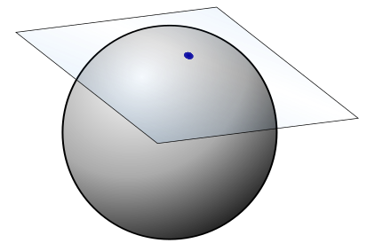
The first major concept in differential geometry is that of a tangent space for a given point on a manifold. Loosely, think of manifold as a space which locally looks like Euclidean space; for example, a sphere in $\mathbb{R}^3$. The tangent space of a manifold is a generalization of the idea of a tangent plane.
Definition: A tangent vector $v_p$ consists of a vector $v$ and a point of application $p$.
There is a natural way to add tangent vectors at a point and multiply them by scalars.
Definition: If two tangent vectors have the same vector $v$ but different points of application, they are said to be parallel.
The best explanation I’ve seen of tangent vectors is by analogy with the concept of a force in physics. A force applied at different areas of a rod will have different results. For example, applied at the midpoint we have translation; applied at the endpoint we have rotation.
Definition: The tangent space $T_p(\mathbb{R}^3)$ is the space consisting of all tangent vectors applied at p.
For convenience sake, we also define the natural frame field on $\mathbb{R^3}$, which consists of the vector fields $U_i$ which are defined so that at every point, $U_i$ returns the $i$th coordinate of the point.
Directional Derivatives
We also define directional derivatives, which we recall from multivariable calculus. The directional derivative in the direction of $v$ is the rate of change along a specific direction $v$.
Definition: The directional derivative of $f$ in the direction of $v$ at a point $p$ is denoted $v_p[f]$.
We can calculate it using the gradient:
$$v_p[f] = \nabla f(p) \cdot \frac{v}{\vert v \vert}$$
And as we would expect, $v_p[f]$ is linear in both $v_p$ and $f$, and the Leibniz rule (product rule) applies as well. No matter what form differentiation takes, we can pretty much always count on linearity and the Leibniz property to hold. We can generalize the idea of a directional derivative to define the operation of a vector field on a function.
Definition: Define the operation $V[f]$ of a vector field $V$ on a function $f$ at each point as follows: $V[f] = V(p)[f]$. In other words, at each point $p$, this construction takes on the value of the directional direvative of $f$ at $p$ in the direction of $V(p)$.
It is clear that $V[f]$ is linear both in $V$ and $f$ and also follows the Leibniz rule, with scalar multiplication defined as usual.
Curves in $\mathbb{R}^3$
We define a curve as a map $\alpha: I\rightarrow \mathbb{R}^3$, where $I$ is an open interval of the real line. We can also define a reparametrization $\beta: J\rightarrow \mathbb{R}^3$ if we define a suitable function $h: J \rightarrow I$.
Indeed, we can think of $\alpha’(t)$ as a collection of tangent vectors defined at each point $\alpha(t)$, and if we do so we can compute directional derivatives. For example, at a given point $\alpha’(t)$, we can define the following directional derivative:
$$\alpha'(t)[f] = \frac{d}{dt} f(\alpha(t))$$
We can prove the above statement using the chain rule. We are applying a tangent vector $\alpha’(t)$ at a point $\alpha(t)$; in other words, at each point of a curve, we compute the directional derivative at that point in the direction of the velocity of the curve. This is a way of computing the rate of change of $f$ “along” the curve $\alpha(t)$.
Defining 1-Forms
Recall the definition of the total derivative from multivariable calculus.
$$ df = \frac{\partial f}{\partial x}dx + \frac{\partial f}{\partial y}dy + \frac{\partial f}{\partial z}dz $$
We’re going to unpack what this really means and finally get around to a rigorous definition of the $dx$ and $dy$ terms we work with everywhere in calculus. Intuitively, $dx$ and $dy$ refer to an infinitesimal quantity in the $x$ and $y$ directions, respectively. We will generalize this notion.
Definition: A 1-form is a linear real-valued function on a tangent space. Thus, a 1-form is an element of the dual space of $T_p (\mathbb R)^3$.
So we can think of 1-forms as functions which send vectors to real numbers. Naturally, we can define the action of a 1-form on a vector field; 1-forms send vector fields to real-valued functions. If you’re reminded of the divergence at this point, you’re on the right track. We now define the most important 1-form of them all:
Definition: The differential of a function $df$ is a 1-form which acts as follows on vectors in a tangent space:
$$ df(v_p) = v_p[f] $$
So, we can think of $df$ as a 1-form which sends each tangent vector to the directional derivative in the direction of the tangent vector. Now we can finally rigorously define $dx, dy, dz$.
Example
Let’s look at the differential $dx$ as a 1-form. From our definitions above, the action of $dx$ on a tangent vector is as follows (here we omit the point of application):
$$ dx = v[x] = \frac{dx}{dx}v_1 + \frac{dx}{dy}v_2 + \frac{dx}{dz}v3 = v_1 $$
In terms of the gradient:
$$ dx = v[x] = (1,0,0) \cdot v = v_1 $$
In other words, the differential $dx$ is a function which sends a vector to the directional derivative of $x$ (whose gradient is defined as the unit vector $\hat{x}$ everywhere) in the direction of $v$.
In this way, we can naturally define a “basis” for the set of all 1-forms as $dx$, $dy$, and $dz$. Any 1-form $\phi$ can be written $\phi = \sum\limits_{i} f_i dx_i$, with $f_i$ named the Euclidean coordinate functions of $\phi$. In Euclidean 3 space, a 1-form is nothing more than a construction of the form:
$$ fdx + gdy + hdz $$
And it is a function from tangent vectors to real numbers. It should also be clear that the differential operator $d$ is linear and satisfies the Leibniz and chain rules. And finally, we can define the differential $df$ in terms of partial derivatives:
$$df = \frac{\partial f}{\partial x}dx + \frac{\partial f}{\partial y}dy + \frac{\partial f}{\partial z}dz$$
And indeed, applying this differential at a point returns the gradient’s projection along that point.
Example
Let’s take a look at the function $f = (x^2 - 1)y + (y^2 + 2)z$. We could use the “partial derivative” definition of f, or instead use the product rule on its factors. In this example:
$$\begin{aligned} df &= (2x\ dx)y + (x^2-1)\ dy + (2y\ dy)z + (y^2+2)\ dz \\ &= 2xy\ dx + (x^2 + 2yz + 1)\ dy + (y^2+2)\ dz \end{aligned}$$
And we can evaluate this differential on a tangent vector $v_p$ as follows:
$$df(v_p) = (2p_1p_2, p_1^2 + 2p_2p_3 +1, p_2^2 + 2) \cdot (v_1, v_2, v_3)$$
In other words, we evaluated the coordinate functions at $p$, and calculated the projection along $v$.
Exterior Derivatives and the Wedge Product
We talked about differential 1-forms, but we can also have differential k-forms for any k. However, when computing products, we have to note that they are anticommutative. For example:
$$ dxdy = -dydx $$
As an immediate consequence, $dxdx = 0$. Thus, 2-forms consist of terms of the form $fdxdy + gdxdz + hdydz$, and all 3-forms are in the form of $fdxdydz$. With the wedge product, we can multiply 1-forms together (thus obtaining a 2-form) term by term.
Definition: Suppose we have a 1-form $\phi$ on $\mathbb{R}^3$. We define its exterior derivative as the 2-form $d\phi = \sum df_i \wedge dx_i$.
Example
Define the 1-form $\phi = xydx + x^2 dz$. We can compute its exterior derivative term by term:
$$ \begin{aligned} d\phi &= d(xy) \wedge dx + d(x^2) \wedge dz \\ &= (y\ dx + x\ dy) \wedge dx + (2x\ dx) \wedge dz \\ &= -x\ dxdy + 2x\ dxdz \end{aligned} $$
In fact, we did not even really need to calculate the $y\ dx$ term, as we knew beforehand that it would disappear with the wedge product.
The exterior derivative, much like the differential and the directional derivative, is linear and follows a modified Leibniz rule across the wedge product:
$$ d(\phi \wedge \psi) = d\phi \wedge \psi - \phi \wedge d\psi $$
Which makes sense given the nature of the wedge product.
Div, Grad and Curl
Now that we have defined wedge products and exterior derivatives, we are ready to express the 3 main operations of differential calculus succinctly in our new notation! Note that the tangent space at $p \in \mathbb{R}^3$ is isomorphic to $\mathbb{R}^3$, so we can choose to define a basis $dx,dy,dz$ as a basis for the tangent space, with the natural isomorphism $\hat{x} \rightarrow dx$ etcetera.
Gradient
First, we define a real-valued function $f$ as a 0-form. Then we take a look at the gradient (which is a 1-form):
$$ \begin{aligned} \nabla f &= \frac{\partial f}{\partial x}\ dx + \frac{\partial f}{\partial y}\ dy + \frac{\partial f}{\partial z}\ dz\\ &= df \end{aligned} $$
Curl
We move on to an understanding of the curl of a vector field $F = (U, V, W)$. We can read $F$ as a 1-form, i.e. $F = U\ dx + V\ dy + W\ dz$. Then, we arrive at the following (using subscript notation for partial derivatives for convenience):
$$ \begin{aligned} dF &= dU \wedge dx + dV \wedge dy + dW \wedge dz \\ &= (U_y - V_x)\ dxdy + (U_z - W_x)\ dxdz + (V_z - W_y)\ dy dz \\ &= \text{curl} F \end{aligned} $$
So, we can think of the curl as the exterior derivative of a 1-Form, read as a two form.
Divergence
We can similarly define the divergence for a vector field $F = (U,V,W)$. First, we read $F$ as a 2-form, in other words:
$$F = U\ dydz - V\ dxdz + W\ dxdy$$
Then, we take a look at the exterior derivative $dF$:
$$ \begin{aligned} dF &= \frac{\partial U}{\partial x}\ dxdydz + \frac{\partial V}{\partial y}\ dxdydz + \frac{\partial W}{\partial z}\ dxdydz \\ &= \text{div}F\ dxdydz \end{aligned} $$
You might be wondering about the minus sign in the second term of our construction of the divergence. That will be taken care of with Hodge duality, when we establish a more explicit correspondence between 1-forms and 2-forms. Loosely, however, we can say this: the gradient takes a 0-form to a one form (vector field); the divergence takes a 1-form to a 2-form (vector field); and the divergence takes a 2-form to a three form (function).
Mappings
Definition: Given a function $F:\mathbb{R}^n \rightarrow \mathbb{R}^m = (f_1(p),…,f_m(p))$, we call $f_i$ the Euclidean coordinate functions of $F$.
Definition: A mapping is a differentiable function from $\mathbb{R}^n$ to $\mathbb{R}^m$.
Using mappings, we can send curves in one space to curves in another space.
Definition: Let $\alpha: I \rightarrow \mathbb{R}^n$ be a curve. Given a mapping $F$, we define the composite function $\beta = F(\alpha): I \rightarrow \mathbb{R}^m$ as the image of $\alpha$ under $F$.
We will study one specific mapping in particular:
Definition: Given a mapping $F:\mathbb{R}^n \rightarrow \mathbb{R}^m$, we define the tangent map to be the following tangent vector at $F(p)$:
$$F_\star (v) = (v[f_1],...,v[f_m]) $$
If we fix a point $p$, we can see that the tangent map $F \star$ sends tangent vectors at $p$ to tangent vectors at $F(p) \in \mathbb{R}^m$. The tangent map is linear in $v$, and furthermore it turns out that The tangent map is the linear transformation that best approximates $F$ at $p$. As a consequence of this, we can prove that tangent maps preserve velocities of curves:
Proof:
Suppose $F=(f_1, f_2, f_3)$. Then we consider the image $\beta$ of a curve $\alpha$ under $F$. $F_\star$ sends a tangent vector at $\alpha(t)$ to a tangent vector at $\beta(t)$
$$ \begin{aligned} F_{\star}(\alpha') &= (\alpha'[f_1], \alpha'[f_2], \alpha'[f_3]) \\ &= \frac{d}{dt}(f_1(\alpha), f_2(\alpha), f_3(\alpha)) \\ =\beta'(t) \end{aligned} $$
Finally, we consider the tangent map applied to a particular type of vector field, the the coordinate maps $U_j$. We use the definition of tangent maps to arrive at:
$$ \begin{aligned} F_{\star}(U_j) = (U_j[f_1], U_j[f_2],...,U_j[f_m]) \end{aligned} $$
And recall that $U_j[f_i] = \frac{\partial f_i}{x_j}$, so we finally arrive at:
$$ \begin{aligned} F_{\star}(U_j) = \sum\limits_{i=1}^m \frac{\partial f_i}{x_j} \hat{U_j} \end{aligned} $$
Where $\hat{U_j}$ refer to the coordinate maps of the codomain $\mathbb{R}^m$. This construction may look familiar; indeed $F_\star(U_j)$ is the $j$th column of the Jacobian matrix of $F$.
Definition: A mapping is regular if at every point in the domain, the tangent map is one-to-one.
We also know that tangent maps are linear transformations, so we can use results from matrices to analyze the above statement. For example, regular maps have tangent maps with a nullspace of exactly $0$.
We can do a lot just with the idea of a tangent vector, which is defined as a pair consisting of a vector and a point of application. The duals of tangent vectors are 1-forms, and we can generalize those to k-forms equipped with a natural addition and scalar multiplication. The exterior derivative works as a generalization of differentiation which maps 1-forms to 2-forms, etc; the velocity curve works as a generalization of the derivative to curves; and finally, the tangent map is a generalization of the derivative to mappings.
Download this Page as a PDF:
Note: Images are replaced by captions.
Recent Posts
- A Note on the Variation of Parameters Method | 11/01/17
- Group Theory, Part 3: Direct and Semidirect Products | 10/26/17
- Galois Theory, Part 1: The Fundamental Theorem of Galois Theory | 10/19/17
- Field Theory, Part 2: Splitting Fields; Algebraic Closure | 10/19/17
- Field Theory, Part 1: Basic Theory and Algebraic Extensions | 10/18/17